A Blender add-on for mathematics and quantitative modelling
Type the model. See it in 3D.
Lab4IQM turns Blender into a mathematics laboratory. You type a command; Python computes the answer exactly where it can; Blender draws it as a surface, a curve or a field you can turn in your hand.
import multicalc
divthm(F=(x, y, z^2), z=0..2, r=0..1, theta=0..2*pi)
F = <x, y, z^2>, div F = 2*z + 2
  int int int div F dV = int_(0)^(2*pi) int_(0)^(1) int_(0)^(2) r*(2*z + 2) dz dr dtheta
  int_(0)^(2) r*(2*z + 2) dz = [r*(z^2 + 2*z)]_(0)^(2) = 8*r
  int_(0)^(1) 8*r dr = [4*r^2]_(0)^(1) = 4
  int_(0)^(2*pi) 4 dtheta = [4*theta]_(0)^(2*pi) = 8*pi
  triple integral = 8*pi = 25.1327
  outward flux through the boundary surface = 8*pi = 25.132741
  the two sides agree
7 modules · 182 commands
Modules
Each module follows a textbook or a field chapter by chapter, with a PDF guide that says which command goes with which section.
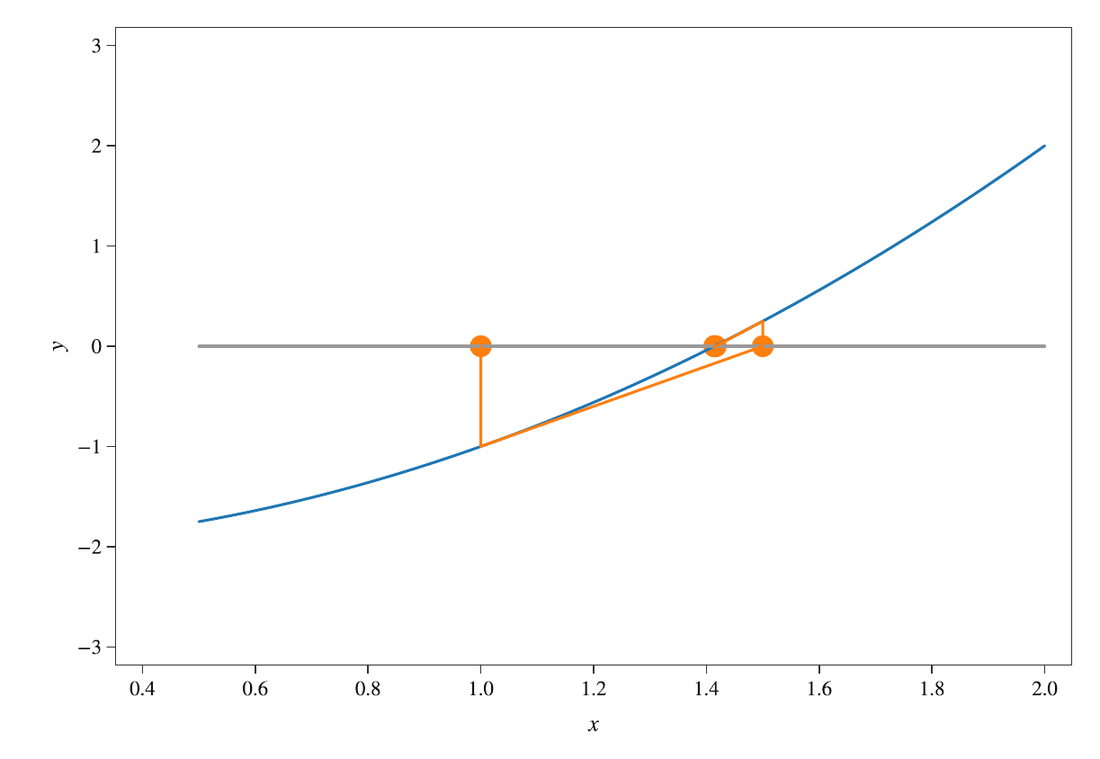
Differential Calculus
0.2.1Functions, limits, derivatives and their applications, with practice problems and answer checking.
OpenStax Calculus Volume 1, Chapters 1–4
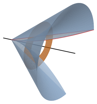
Integral Calculus
1.0.0Integrals and their applications, techniques of integration, differential equations, sequences and series, power series, parametric and polar curves.
OpenStax Calculus Volume 2, Chapters 1–7
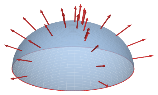
Multivariable Calculus
1.0.0Vectors and space curves, partial derivatives, multiple integrals, vector calculus with the theorems of Green, Stokes and Gauss, and second-order differential equations.
OpenStax Calculus Volume 3, Chapters 2–7
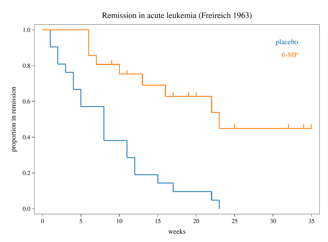
Biostatistics
0.1.2Survival curves with the log-rank test, ROC curves, group comparisons, contingency tables and dose–response fits, from a CSV file.
Results checked against R and published values
Mathematical Oncology
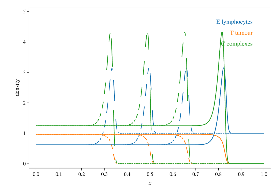
0.3.0Tumour growth, spheroids, tissue mechanics, immune response, angiogenesis, invasion and metastasis: the models solved and drawn.
Follows Chaplain & Preziosi, Chapters 2–11
Graph Theory
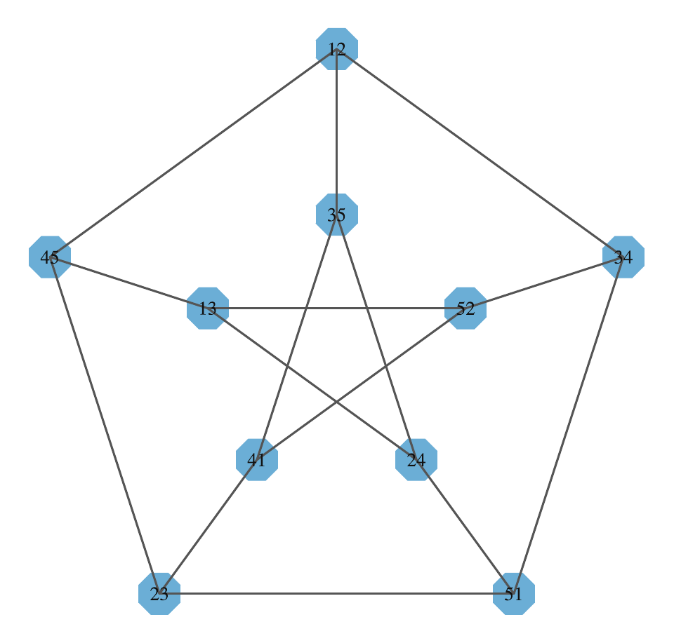
0.2.0Graphs drawn in 2D and 3D, isomorphism, cycles, decompositions, Eulerian circuits, degree sequences and directed graphs.
Follows West, Introduction to Graph Theory, Chapter 1
Computational Topology
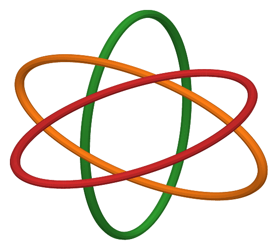
0.3.0Knots, surfaces and complexes, homology, duality, Morse theory and persistent homology, computed and shown in 3D.
Follows Edelsbrunner & Harer, Computational Topology, Chapters I–VIII
Next
A module for your course
Modules follow a textbook or a syllabus chapter by chapter. If you teach a quantitative subject and want one for your course, write with the book and the chapters you use.
More chapters of the modules in progress are on the way.
How it works
Python computes
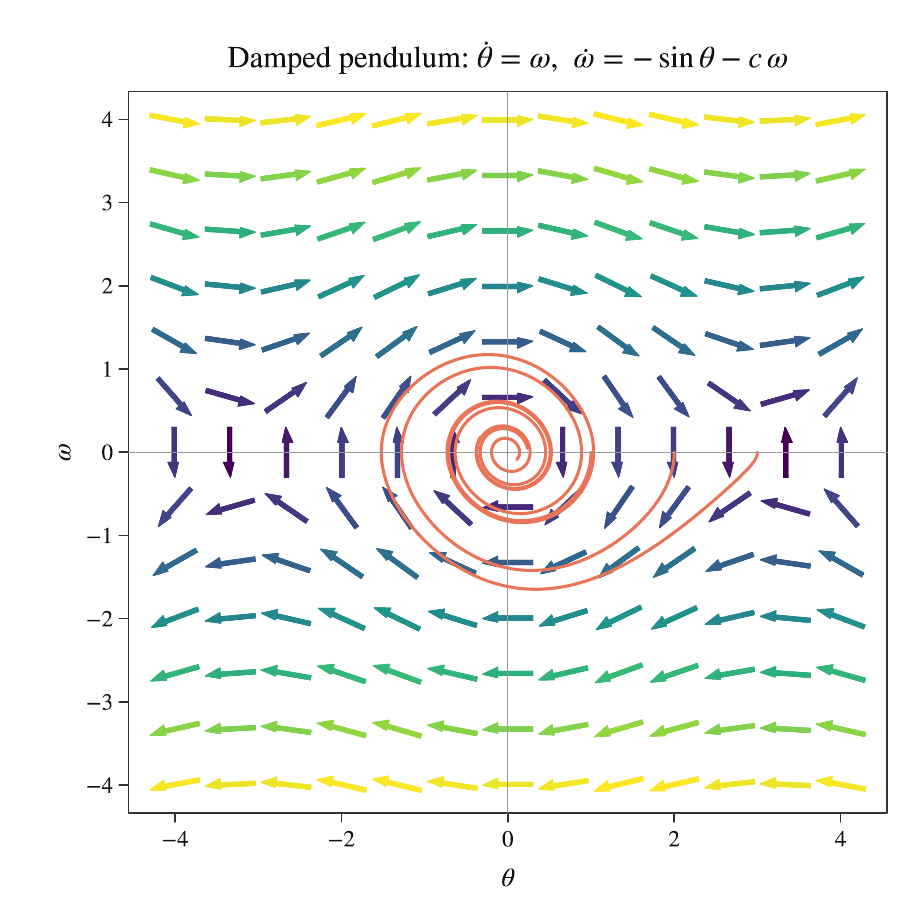
A pure Python and NumPy core does the mathematics, including its own symbolic engine for derivatives, integrals, limits and series. Each step is printed, the way you would write it.
Blender draws
Results become real 3D objects: surfaces, solids of revolution, vector fields, graphs and knots. Turn them, light them, export them as PDF figures for a paper or render them for a talk.
Answers are checked
Exact answers are compared with a numerical computation done a different way,
and every module ships with its tests. Students can test their own answers with check(...).
For teaching and for research
From a first calculus course to a research figure
Students use the calculus modules beside their textbook: every section has commands that draw its ideas,
practice problems generated at random, and a check command that says what went wrong in their answer.
Researchers write models in a Python script, see them while they work, and compile a LaTeX paper whose figures update with the model.
- Console commands and Python scripts work side by side.
- Vector PDF and SVG export for papers; rendered images for slides.
- LaTeX documents compiled inside Blender, figures included by name.